
How To Read an Unlabeled Sales Chart
By Evan Miller
February 4, 2013
A genre of blog post that is perennially popular among independent software developers is “How My Sales Skyrocketed After…”, where for the ellipsis you my substitute any number of fortuitous events or marketing techniques.
I thought about contributing to this literature after one of my apps was recently subjected to a fortuitous event that markedly increased sales. I imagined regaling the reader with vivid tales of toil and hardship that inevitably culminated in a bar chart with its Y-axis blurred out.
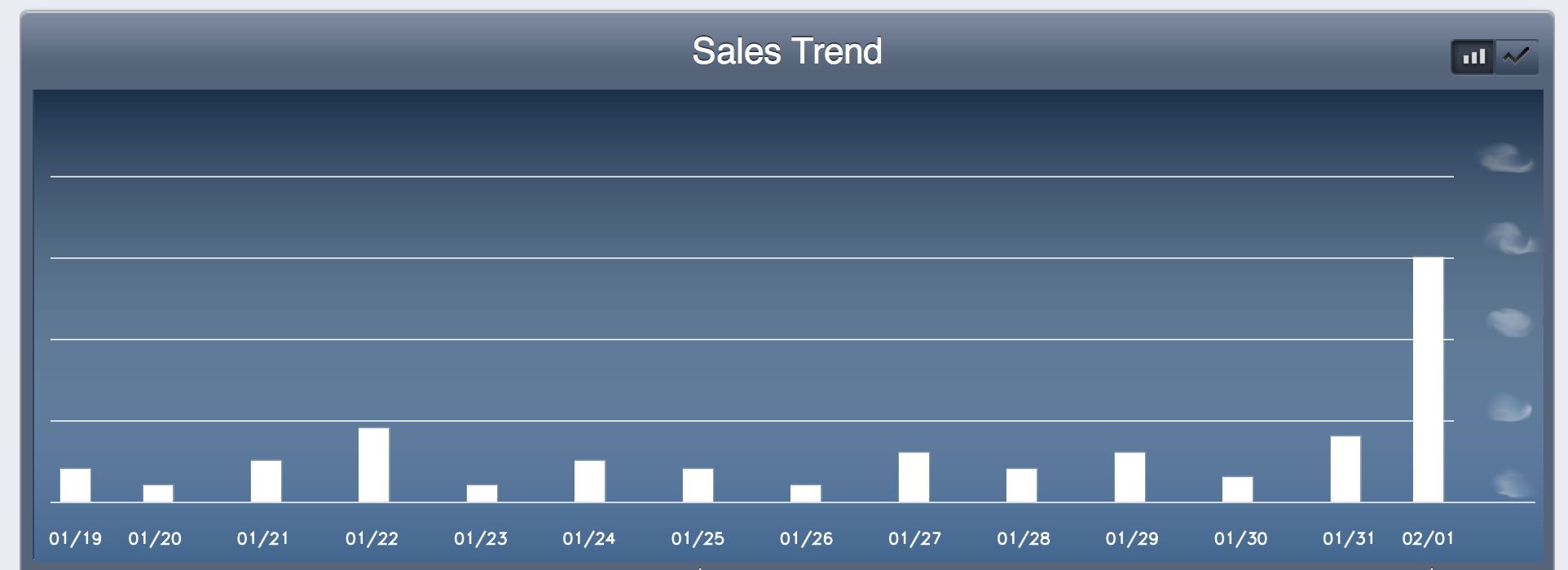
Figure 1: Sales chart with its Y-axis blurred out.
As I pondered the blurred-out Y-axis in the above picture, a much more interesting topic occurred to me, and so I’ve decided to write about that instead: how to deduce the scale of a sales chart in which the Y-axis is missing.
The following techniques only work for charts that represent counts of some sort; if the Y-axis is a continuous measurement, you’ll need to find another blog to read. There’s a little bit of math here, but you can do the important bits in a spreadsheet program.
Technique #1: Counting Pixels and the Riemann Zeta Function
The first thing you might try is to measure the size of each bar in pixels and determine the greatest common divisor among all of the pixel counts. If there is no common divisor among the sale counts, then greatest common divisor among the pixel counts will correspond to the number of pixels that represent a single sale.
If you have two weeks’ worth of data, the odds are actually pretty good that the sale counts won’t have a common divisor. In fact the probability can be approximated as:
\[ [\zeta(14)]^{-1} = 0.9999388\ldots \]That’s the multiplicative inverse of the Riemann zeta function, which can be used to estimate the probability that a number of randomly chosen integers have no common divisor. Here I used 14 since there are 14 bars in a two-week chart. Here’s a table with more values (the Riemann zeta, unfortunately, is not implemented in Excel):
| N | [ζ(N)]-1 |
|---|---|
| 2 | 0.607927 |
| 4 | 0.923938 |
| 6 | 0.982953 |
| 8 | 0.995939 |
| 10 | 0.999006 |
| 12 | 0.999754 |
| 14 | 0.999939 |
The left column corresponds to the number of integers in a given sample; the right column gives the probability that there is no common divisor among the same number of randomly chosen integers. (That is, the probability that this technique will work correctly.)
Of course, this technique won’t work at all if the picture is too blurry or if there could be more than one sale per pixel. In those situations we’ll need to impose a little more structure on the problem.
Technique #2: Properties of a Poisson Process
In the absence of calamity, fortuitous events, or brilliant new marketing strategies, sale counts are well-described by a Poisson process. That is, you can think of there being an underlying average number of sales per day, and each day will be a realization of a Poisson distribution with that average.
The neat thing about a Poisson distribution is that its mean is equal to its variance. We can exploit this simple fact to estimate the scale of a missing Y-axis.
Suppose we have a measurement of each bar’s height in pixels: \(\{P_1, P_2, \ldots, P_N\}\), with an average height \(\bar{P}\). Let \(S\) be the number of sales per pixel. Assuming sales are a Poisson process, we can equate the sales mean to the sales variance:
\[ S \bar{P} = \frac{1}{n-1} \sum_{i=1}^N(S P_i - S \bar{P})^2 \]Rearranging you get a nice equation for sales per pixel:
\[ S = \frac{(n-1)\bar{P}}{\sum_{i=1}^N (P_i - \bar{P})^2} \]Which could also be written:
\[ S = \frac{\bar{P}}{Var(P)} \]In plain English, the number of sales per pixel can be estimated as the average bar height in pixels divided by the variance of the bar heights.
To see how well this works in practice, I ran the numbers on the first 13 bars of the above chart (that is, before the sales spike, which interrupted the usual Poisson process). The resulting estimate was about 6% different than the actual scale of the Y-axis. I guess my sales figures won’t be a secret for long!
An advantage of this technique is that the pixel measurements here don’t have to be exact, because we only care about the sample mean and variance. In fact we don’t have to measure pixels at all; any unit of measurement will do. Unlike in Technique #1 above, where we were computing greatest common divisors among sets of integers, the exact integer values of individual measurements are not crucial in order to obtain an accurate order-of-magnitude estimate.
Try it out for yourself. See if you can deduce how much, exactly, my sales skyrocketed after…
You’re reading evanmiller.org, a random collection of math, tech, and musings. If you liked this you might also enjoy:
Get new articles as they’re published, via LinkedIn, Twitter, or RSS.
Want to look for statistical patterns in your MySQL, PostgreSQL, or SQLite database? My desktop statistics software Wizard can help you analyze more data in less time and communicate discoveries visually without spending days struggling with pointless command syntax. Check it out!

Back to Evan Miller’s home page – Subscribe to RSS – LinkedIn – Twitter