Statistical Formulas For Programmers
By Evan Miller
May 19, 2013
Being able to apply statistics is like having a secret superpower.
Where most people see averages, you see confidence intervals.
When someone says “7 is greater than 5”, you declare that they’re really the same.
In a cacophony of noise, you hear a cry for help.

Unfortunately, not enough programmers have this superpower. That’s a shame, because the application of statistics can almost always enhance the display and interpretation of data.
As my modest contribution to developer-kind, I’ve collected together the statistical formulas that I find to be most useful; this page presents them all in one place, a sort of statistical cheat-sheet for the practicing programmer.
Most of these formulas can be found in Wikipedia, but others are buried in journal articles or in professors’ web pages. They are all classical (not Bayesian), and to motivate them I have added concise commentary. I’ve also added links and references, so that even if you’re unfamiliar with the underlying concepts, you can go out and learn more. Wearing a red cape is optional.
Send suggestions and corrections to emmiller@gmail.com
Table of Contents
- Formulas For Reporting Averages
- Formulas For Reporting Proportions
- Formulas For Reporting Count Data
- Formulas For Comparing Distributions
- Formulas For Drawing a Trend Line
1. Formulas For Reporting Averages
One of the first programming lessons in any language is to compute an average. But rarely does anyone stop to ask: what does the average actually tell us about the underlying data?
1.1 Corrected Standard Deviation
The standard deviation is a single number that reflects how spread out the data actually is. It should be reported alongside the average (unless the user will be confused).
\[ s = \sqrt{\frac{1}{N-1} \sum_{i=1}^N(x_i - \bar{x})^2} \]Where:
- \(N\) is the number of observations
- \(x_i\) is the value of the \(i\)th observation
- \(\bar{x}\) is the average value of \(x_i\)
Reference: Standard deviation (Wikipedia)
1.2 Standard Error of the Mean
From a statistical point of view, the "average" is really just an estimate of an underlying population mean. That estimate has uncertainty that is summarized by the standard error.
\[ SE = \frac{s}{\sqrt{N}} \]Reference: Standard error (Wikipedia)
1.3 Confidence Interval Around the Mean
A confidence interval reflects the set of statistical hypotheses that won’t be rejected at a given significance level. So the confidence interval around the mean reflects all possible values of the mean that can’t be rejected by the data. It is a multiple of the standard error added to and subtracted from the mean.
\[ CI = \bar{x} \pm t_{\alpha/2} SE \]Where:
- \(\alpha\) is the significance level, typically 5% (one minus the confidence level)
- \(t_{\alpha/2}\) is the \(1-\alpha/2\) quantile of a t-distribution with \(N-1\) degrees of freedom
Reference: Confidence interval (Wikipedia)
1.4 Two-Sample T-Test
A two-sample t-test can tell whether two groups of observations differ in their mean.
The test statistic is given by:
\[ t = \frac{\bar{x_1} - \bar{x_2}}{\sqrt{s^2_1/n_1 + s^2_2/n_2}} \]The hypothesis of equal means is rejected if \(|t|\) exceeds the \((1-\alpha/2)\) quantile of a t distribution with degrees of freedom equal to:
\[ {\rm df} = \frac{(s_1^2/n_1+s_2^2/n_2)^2}{(s_1^2/n_1)^2/(n_1-1)+(s_2^2/n_2)^2/(n_2-1)} \]You can see a demonstration of these concepts in Evan’s Awesome Two-Sample T-Test.
Reference: Student’s t-test (Wikipedia)
2. Formulas For Reporting Proportions
It’s common to report the relative proportions of binary outcomes or categorical data, but in general these are meaningless without confidence intervals and tests of independence.
2.1 Confidence Interval of a Bernoulli Parameter
A Bernoulli parameter is the proportion underlying a binary-outcome event (for example, the percent of the time a coin comes up heads). The confidence interval is given by:
\[ CI = \left(p + \frac{z^2_{\alpha/2}}{2N} \pm z_{\alpha/2} \sqrt{[p(1-p) + z^2_{\alpha/2}/4N]/N}\right)/(1+z^2_{\alpha/2}/N) \]Where:
- \(p\) is the observed proportion of interest
- \(z_{\alpha/2}\) is the \((1-\alpha/2)\) quantile of a normal distribution
This formula can also be used as a sorting criterion.
Reference: Binomial proportion confidence interval (Wikipedia)
2.2 Multinomial Confidence Intervals
If you have more than two categories, a multinomial confidence interval supplies upper and lower confidence limits on all of the category proportions at once. The formula is nearly identical to the preceding one.
\[ CI = \left(p_j + \frac{z^2_{\alpha/2}}{2N} \pm z_{\alpha/2} \sqrt{[p_j(1-p_j) + z^2_{\alpha/2}/4N]/N}\right)/(1+z^2_{\alpha/2}/N) \]Where:
- \(p_j\) is the observed proportion of the \(j\)th category
Reference: Confidence Intervals for Multinomial Proportions
2.3 Chi-Squared Test
Pearson’s chi-squared test can detect whether the distribution of row counts seem to differ across columns (or vice versa). It is useful when comparing two or more sets of category proportions.
The test statistic, called \(X^2\), is computed as:
\[ X^2 = \sum_{i=1}^{n}\sum_{j=1}^m \frac{(O_{i,j} - E_{i,j})^2}{E_{i,j}} \]Where:
- \(n\) is the number of rows
- \(m\) is the number of columns
- \(O_{i,j}\) is the observed count in row \(i\) and column \(j\)
- \(E_{i,j}\) is the expected count in row \(i\) and column \(j\)
The expected count is given by:
\[ E_{i,j} = \frac{\sum_{k=1}^nO_{k,j} \sum_{l=1}^mO_{i,l} }{N} \]Where:
- \(N\) is the sum of all the cells, i.e., the total number of observations
A statistical dependence exists if \(X^2\) is greater than the (\(1-\alpha\)) quantile of a \(\chi^2\) distribution with \((m-1)\times(n-1)\) degrees of freedom.
You can see a 2x2 demonstration of these concepts in Evan’s Awesome Chi-Squared Test.
Reference: Pearson’s chi-squared test (Wikipedia)
3. Formulas For Reporting Count Data
If the incoming events are independent, their counts are well-described by a Poisson distribution. A Poisson distribution takes a parameter \(\lambda\), which is the distribution’s mean — that is, the average arrival rate of events per unit time.
3.1. Standard Deviation of a Poisson Distribution
The standard deviation of Poisson data usually doesn’t need to be explicitly calculated. Instead it can be inferred from the Poisson parameter:
\[ \sigma = \sqrt{\lambda} \]This fact can be used to read an unlabeled sales chart, for example.
Reference: Poisson distribution (Wikipedia)
3.2. Confidence Interval Around the Poisson Parameter
The confidence interval around the Poisson parameter represents the set of arrival rates that can’t be rejected by the data. It can be inferred from a single data point of \(c\) events observed over \(t\) time periods with the following formula:
\[ CI = \left(\frac{\gamma^{-1}(\alpha/2, c)}{t}, \frac{\gamma^{-1}(1-\alpha/2, c+1)}{t}\right) \]Where:
- \(\gamma^{-1}(p, c)\) is the inverse of the lower incomplete gamma function
Reference: Confidence Intervals for the Mean of a Poisson Distribution
3.3. Conditional Test of Two Poisson Parameters
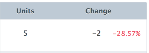
Please never do this:

From a statistical point of view, 5 events is indistinguishable from 7 events. Before reporting in bright red text that one count is greater than another, it’s best to perform a test of the two Poisson means.
The p-value is given by:
\[ p = 2\times\frac{c!}{t^c}\times\min\left\{ \sum_{i=0}^{c_1} \frac{t_1^i t_2^{c-i}}{i!(c-i)!}, \sum_{i=c_1}^{c} \frac{t_1^i t_2^{c-i}}{i!(c-i)!} \right\} \]Where:
- Observation 1 consists of \(c_1\) events over \(t_1\) time periods
- Observation 2 consists of \(c_2\) events over \(t_2\) time periods
- \(c = c_1 + c_2\) and \(t = t_1 + t_2\)
You can see a demonstration of these concepts in Evan’s Awesome Poisson Means Test.
Reference: A more powerful test for comparing two Poisson means (PDF)
4. Formulas For Comparing Distributions
If you want to test whether groups of observations come from the same (unknown) distribution, or if a single group of observations comes from a known distribution, you’ll need a Kolmogorov-Smirnov test. A K-S test will test the entire distribution for equality, not just the distribution mean.
4.1. Comparing An Empirical Distribution to a Known Distribution
The simplest version is a one-sample K-S test, which compares a sample of \(n\) points having an observed cumulative distribution function \(F\) to a known distribution function having a c.d.f. of \(G\). The test statistic is:
\[ D_n = \sup_x|F(x) - G(x)| \]In plain English, \(D_n\) is the absolute value of the largest difference in the two c.d.f.s for any value of \(x\).
The critical value of \(D_n\) at significance level \(\alpha\) is given by \(K_\alpha/\sqrt{n}\), where \(K_\alpha\) is the value of \(x\) that solves:
\[ 1 - \alpha = \frac{\sqrt{2\pi}}{x}\sum_{k=1}^\infty \exp{\left(-(2k-1)^2\pi^2/(8x^2)\right)} \]The critical must be solved iteratively, e.g. by Newton’s method. If only the p-value is needed, it can be computed directly by solving the above for \(\alpha\).
Reference: Kolmogorov-Smirnov Test (Wikipedia)
4.2. Comparing Two Empirical Distributions
The two-sample version is similar, except the test statistic is given by:
\[ D_{n_1,n_2} = \sup_x|F_1(x) - F_2(x)| \]Where \(F_1\) and \(F_2\) are the empirical c.d.f.s of the two samples, having \(n_1\) and \(n_2\) observations, respectively. The critical value of the test statistic is \(K_\alpha/\sqrt{n_1 n_2/(n_1 + n_2)}\) with the same value of \(K_\alpha\) above.
Reference: Kolmogorov-Smirnov Test (Wikipedia)
4.3. Comparing Three or More Empirical Distributions
A \(k\)-sample extension of Kolmogorov-Smirnov was described by J. Kiefer in a 1959 paper. The test statistic is:
\[ T = \sup_x \sum_{j=1}^k n_j |F_j(x) - \bar{F}(x)| \]Where \(\bar{F}\) is the c.d.f. of the combined samples. The critical value of \(T\) is \(a^2\) where \(a\) solves:
\[ 1 - \alpha = \frac{4}{\Gamma\left(\frac{h}{2}\right)2^{h/2}a^h} \sum_{n=1}^\infty \frac{(\gamma_{(h-2)/2,n})^{h-2}\exp[-(\gamma_{(h-2)/2,n})^2/2a^2]}{[J_{h/2}(\gamma_{(h-2)/2,n})]^2} \]Where:
- \(h=k-1\)
- \(J_{h/2}\) is a Bessel function of the first kind with order \(h/2\)
- \(\gamma_{(h-2)/2,n}\) is the \(n\)th zero of \(J_{(h-2)/2}\)
To compute the critical value, this equation must also be solved iteratively. When \(k=2\), the equation reduces to a two-sample Kolmogorov-Smirnov test. The case of \(k=4\) can also be reduced to a simpler form, but for other values of \(k\), the equation cannot be reduced.
Reference: K-sample analogues of the Kolmogorov-Smirnov and Cramer-v. Mises tests (JSTOR)
5. Formulas For Drawing a Trend Line
Trend lines (or best-fit lines) can be used to establish a relationship between two variables and predict future values.
5.1. Slope of a Best-Fit Line
The slope of a best-fit (least squares) line is:
\[ m = \frac{\sum_{i=1}^N(x_i - \bar{x})(y_i - \bar{y})}{\sum_{i=1}^N(x_i - \bar{x})^2} \]Where:
- \(\{x_1, \ldots, x_N\}\) is the independent variable with sample mean \(\bar{x}\)
- \(\{y_1, \ldots, y_N\}\) is the dependent variable with sample mean \(\bar{y}\)
5.2. Standard Error of the Slope
The standard error around the estimated slope is:
\[ SE = \frac{\sqrt{\sum_{i=1}^N(y_i - \bar{y} - m (x_i - \bar{x}))^2/(N-2)}}{\sqrt{\sum_{i=1}^N(x_i - \bar{x})^2}} \]5.3. Confidence Interval Around the Slope
The confidence interval is constructed as:
\[ CI = m \pm t_{\alpha/2} SE \]Where:
- \(\alpha\) is the significance level, typically 5% (one minus the confidence level)
- \(t_{\alpha/2}\) is the \(1-\alpha/2\) quantile of a t-distribution with \(N-2\) degrees of freedom
Reference: Simple linear regression (Wikipedia)
You’re reading evanmiller.org, a random collection of math, tech, and musings. If you liked this you might also enjoy:
Get new articles as they’re published, via LinkedIn, Twitter, or RSS.
Want to look for statistical patterns in your MySQL, PostgreSQL, or SQLite database? My desktop statistics software Wizard can help you analyze more data in less time and communicate discoveries visually without spending days struggling with pointless command syntax. Check it out!
Back to Evan Miller’s home page – Subscribe to RSS – LinkedIn – Twitter

